What Are Data Cubes | OLAP

Since we learned that Apache Kylin works on multi-dimensional cubes paving the path for Online Analytical Processing (OLAP). We now must understand how data cubes work.

What is Data Cube?

A data cube is a lattice of cuboids. A cube is defined as a multidimensional dataset which is also sometimes called a hypercube if the number of dimensions is greater than 3. As the dimensions increase, storage space is excessively needed. So let's first discuss definitions of dimensions and measures in the data cube?

The dimension corresponds to an attribute or a set of attributes in the schema, and each cell stores the value of some aggregate measure such as count or sum.

Types of Aggregate Measures:

COUNT – counts rows in a specified table or view.
AVG – calculates the average of a set of values.
SUM – calculates the sum of values.
MIN – gets the minimum value in a set of values.
MAX – gets the maximum value in a set of values.

To call an aggregate function, you use the following syntax:

aggregate_function (DISTINCT | ALL expression)

Let's take a closer look at the syntax above:

To begin, choose an aggregate function to apply, such as MIN, MAX, AVG, SUM, or COUNT.
Secondly, inside parentheses, place the DISTINCT or ALL modifier followed by an expression. The aggregate function ignores duplicate data and only examines unique values when the DISTINCT modifier is used. When you employ the ALL modifier, the aggregate function calculates or evaluates all values. If no other modifier is specified, the ALL modifier is applied by default.

A data cube for AllElectronics

Consider creating a data cube for AllElectronics sales that includes the following fields: city, item, year, and sales in dollars. You need to be able to analyze the data using queries like these:

"Compute the sum of sales, grouping by city and item."
"Compute the sum of sales, grouping by city."
"Compute the sum of sales, grouping by item."
"Compute the sum of sales, grouping by year."

What is the total number of cuboids, or group-by's, that this data cube can compute? Using the three dimensions of the data cube, city, item, and year, and the measure of sales in dollars, the total number of cuboids, or group-by's, that can be computed for this data cube is 2³ = 8. The following are possible group-bys: (city, item, year), (city, item), (city, year), (item, year), (city), (item), (year), (city), (item), (year), () (i.e., the dimensions are not grouped).

The base cuboid, which contains all three dimensions, city, item, and year, is the least generalized (most specific) of the cuboids. It can give you the total sales for any of the three dimensions. The apex cuboid, also known as the 0-D cuboid, is the most generalized (least specific) of the cuboids, referring to the situation in which the group-by is empty. It has the entire amount of all sales in it. Drilling down within the data cube is analogous to starting at the apex cuboid and exploring downward in the lattice. This is connected to rolling up if we start at the base cuboid and work our way up.

Operations for OLAP queries are:

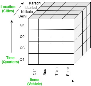
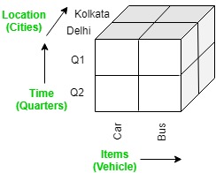
Let's suppose a data cube of VehicleSales Data where dimensions are location, time, and items whereas sales are taken as a measure.

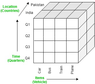
1. Roll-up: This operation takes the current data object and does a further group-by on one of the dimensions. It can be done by:

Climbing up in the hierarchy
Reducing the dimensions

In the diagram below, we have climbed up in the hierarchy of Location dimension (City -> Country).

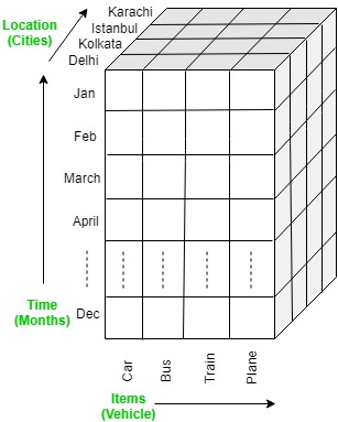
2. Drill-down: As the converse of roll-up, this operation tries to get a more detailed presentation. It can be done by:

Moving down in the hierarchy
Adding a new dimension

For example, In the diagram below, we have gone down the hierarchy of Time dimension (Quarter -> Month).

3. Pivot: It is also known as rotation operation as it rotates the current view to get a new view of the representation.

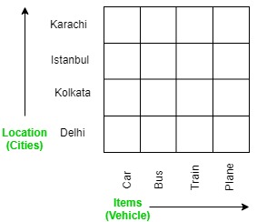
4. Slice: This operation selects a single dimension from the OLAP cube which results in a new sub-cube creation. In the following cube, a Slice is performed on the dimension Time = "Q1".

5. Dice: This operation selects a sub-cube from the OLAP cube by selecting two or more dimensions. A sub-cube is selected by selecting the following dimensions with criteria:

Location = “Delhi” or “Kolkata”
Time = “Q1” or “Q2”
Item = “Car” or “Bus”

Now, moving onwards with the AllElectronics data cube, An SQL query containing no group-by (e.g., "compute the sum of total sales") is a zero-dimensional operation. An SQL query containing one group-by (e.g., “compute the sum of sales, group-by city ”) is a one-dimensional operation. A cube operator on n dimensions is equivalent to a collection of group-by statements, one for each subset of the n dimensions. Therefore, the cube operator is the n-dimensional generalization of the group-by operator. For a cube with n dimensions, there are a total of 2n cuboids, including the base cuboid. A statement such as compute cube sales_cube would explicitly instruct the system to compute the sales aggregate cuboids for all eight subsets of the set {city, item, year }, including the empty subset.

The Curse of Dimensionality

It may seem like a good idea to compute in advance all or at least some of the cuboids in a data cube. Precomputation leads to faster response time and avoids some redundant computation. But we face a major challenge related to this precomputation, which is that the required storage space may explode if all the cuboids in a data cube are precomputed, especially when the cube has many dimensions. The storage requirements are even more excessive when many of the dimensions have associated concept hierarchies, each with multiple levels. This problem is referred to as the curse of dimensionality.

In reality, many dimensions do have hierarchies. For example, time is usually explored not at only one conceptual level (e.g., year), but rather at multiple conceptual levels such as in the hierarchy "day < month < quarter < year". You probably realize that it is unrealistic to precompute all of the cuboids that can possibly be generated for a data cube. If there are many cuboids, and these cuboids are large in size, a more reasonable option is partial materialization; that is, to precompute only some of the possible cuboids that can be generated.

Now, Let's take a close look at the AllElectronic Sales data cube. It has three dimensions: address (with city values Chicago, New York, Toronto, Vancouver), time (with quarter values Q1, Q2, Q3, Q4), and item (with item type values home entertainment, computer, phone, security). The aggregate value stored in each cell of the cube is sales_amount (in thousands). For example, the total sales for the first quarter, Q1, for the items related to security systems in Vancouver is $400,000, as stored in cell 〈Vancouver, Q1, security〉.

Relationship between Data Warehousing and OLAP

Most data warehouses use star schemas to represent the multidimensional data model. In a star schema there is a single fact table (which is at the center of a star schema and contains most of the data stored in the data warehouse), and a set of dimension tables that can be used in combination with the fact table (a single table for each dimension).

The star schema model of data warehouses makes join indexing attractive for cross-table search because the connection between a fact table and its corresponding dimension tables is the foreign key of the fact table and the primary key of the dimension table. Join indexing maintains relationships between attribute values of a dimension and the corresponding rows in the fact table. Join indices may span multiple dimensions to form composite join indices.

Conclusion:

This article explains the detailed concept of a Data Cube and how it works and helps with OLAP functions.

Thanks for reading!